3 Methodology
3.1 Area of Interest - spatial and temporal delimitation
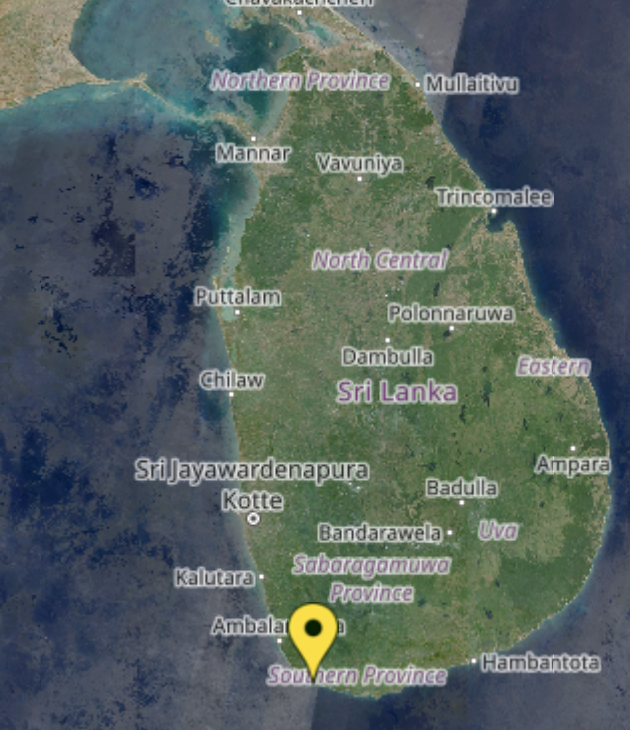
The project focuses on a specific area in Sri Lanka, with particular attention to the coastal region of Unawatuna, as shown in Figure 3.1. The spatial delimitation encompasses a defined area within the coordinates, extending approximately from 6.0048°N, 80.2422°E in the southwest to 6.0112°N, 80.2534°E in the northeast. This area was chosen due to the presence of a distinct sandbank, which provides a clear and measurable feature for analysis. The temporal delimitation of this analysis spans a five-year period from 2019 to 2023, with the goal of identifying any changes in the beach during this timeframe.
3.2 Data acquisition
The satellite data for the project was sourced from Sentinel Hub, covering a 5-year period. The data was downloaded as SAFE files, which is the standard format for Sentinel satellite data. Initially, the complete dataset for the region was acquired. In a subsequent step, the data was cropped to focus specifically on the area of interest.
To ensure data quality, it was crucial to select images captured on clear days with minimal cloud coverage over the target beach area. Each image was manually inspected to verify clarity and relevance before being added to the dataset. This approach ensured that the dataset was reliable and suitable for subsequent analysis.
3.3 Data preprocessing challenges
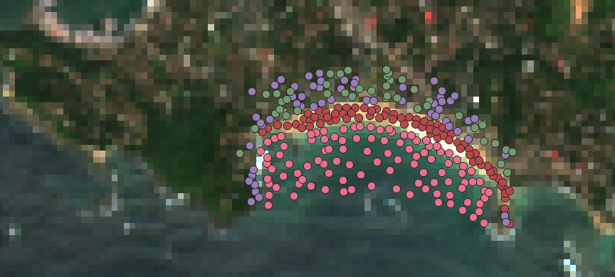
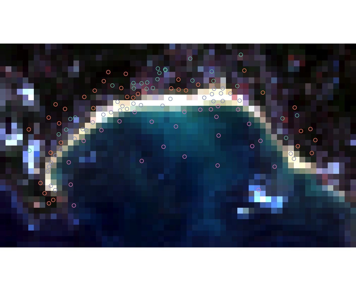
The first step after downloading the satellite images was to manually annotate the data, as no pre-labeled datasets were available, as shown in Figure 3.2. In the absence of preexisting training and testing datasets, manual annotation of the satellite images from Sri Lanka was performed using QGIS.
A GeoPackage layer was created to classify the imagery into four categories: Sand, Buildings, Water, and Forest. These categories were defined based on their distinct spectral levels, which cannot be easily mixed or generalized. By distinguishing between these features, the categorization ensured specificity and improved the accuracy of subsequent analysis.
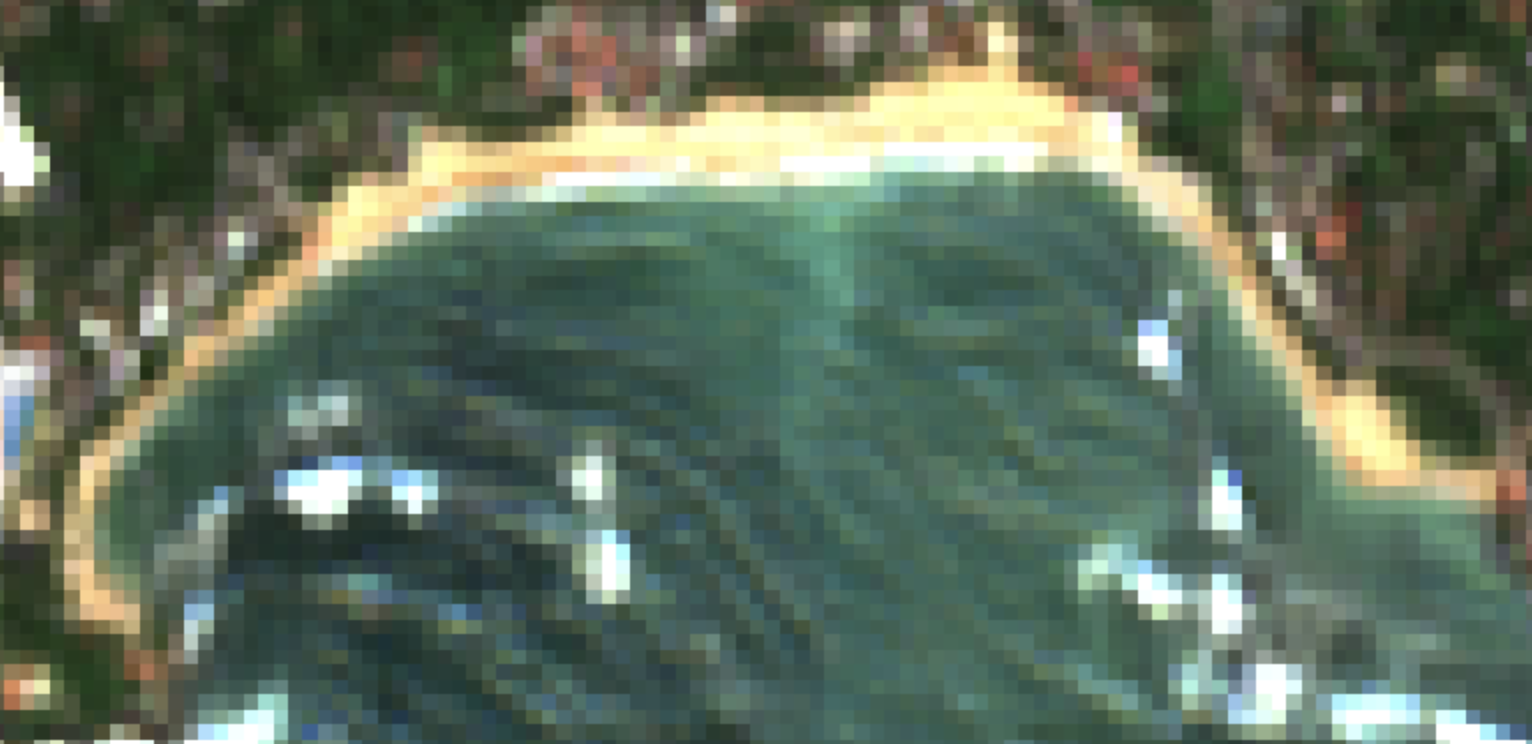
Precise labeling proved challenging due to the low resolution of the downloaded satellite data, which resulted in significant pixelation and made it difficult to reliably differentiate between the categories. To address this issue, high-resolution ESRI satellite imagery was used as a reference to ensure accurate labeling, illustrated in Figure 3.3. However, ESRI imagery is limited to current data and does not provide historical coverage, making it unsuitable for temporal analysis. To complement this, Sentinel-2 data was employed to access a multi-year temporal archive, enabling the analysis of changes over time despite its lower resolution.
The integration of manual geospatial annotation in QGIS, precise class-specific labeling with a GeoPackage, and the inclusion of multiple Sentinel-2 bands laid the groundwork for constructing a comprehensive training dataset. This dataset serves as the foundation for training the machine learning model.
3.4 Resolution
When downloading data from Corpernicus Browser, the SAFE package provides three different spatial resolutions: 10m, 20m, and 60m. However, not all spectral bands are available at all resolutions. Generally, as the spatial resolution increases, fewer bands are included.
For instance, at the 10m resolution, only the following bands are available: B2, B3, B4, and B8. These bands are primarily focused on visible and near-infrared (NIR) light:
B2 (Blue): Sensitive to water bodies and atmospheric corrections.
B3 (Green): Highlights vegetation health and serves as a general-purpose visible band.
B4 (Red): Crucial for vegetation analysis and differentiating between vegetation and soil.
B8 (NIR): This band could be used for the NDVI, which would help to differentiate the borders of the vegetation to the beach.
In contrast, the 20m resolution offers a more comprehensive range of bands, including B1–B8A, B11, and B12. These additional bands provide extended spectral information for more detailed remote sensing analyses, which could help to specify the data (GISGeography 2019):
B5 (Red Edge): This band could be used to detect transition between visible red and near-infrared (NIR). It may help identify shifts in vegetation that interact with dynamic beach environments.
B6 (NIR): This band could provide insights into variations in vegetation structure near the beach.
B7 (NIR): This band could refine the detection of subtle vegetation changes, such as identifying sparse vegetation growth on or near sand dunes, supporting long-term environmental monitoring.
B8A (NIR): This band could enhance the precision of detecting land cover changes, such as transitions between sandy surfaces, vegetation, and human-made structures.
B11 (SWIR 1): This band could be used to detect moisture levels in sandy areas.
B12 (SWIR 2): This band could help distinguish between sand, vegetation, and other surface materials, making it valuable for analyzing erosion patterns and mapping changes in beach morphology.
For the initial analysis, all available bands at the 20m resolution were utilized for training, as the relative importance of individual bands has not yet been determined. This comprehensive approach ensures no potentially relevant spectral information is overlooked, offering flexibility in identifying the most impactful bands for specific applications.
3.5 Dataset: training and test data
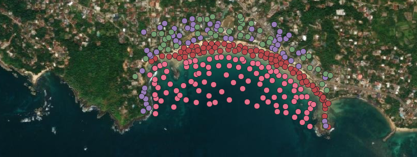
To train the machine learning models, it was essential to create a training dataset, as demonstrated in Figure 3.4. This dataset was generated using a cropped region of Unawatuna, based on a recent satellite image. The training process utilized the entire image from this region to ensure comprehensive coverage. For testing, separate beaches from other regions within the downloaded satellite data of Sri Lanka were selected as the test dataset.
The decision to use test data from the same satellite imagery and within Sri Lanka was based on the need to maintain consistency in environmental features such as vegetation. Vegetation can vary significantly across regions, potentially introducing discrepancies in model accuracy if vastly different environments were used. For instance, buildings in coastal areas like Barcelona differ greatly from those in Sri Lanka. In Barcelona, structures are often taller with flat rooftops, while in Sri Lanka, houses typically have red-tiled roofs and are shorter.
The test dataset comprised two different beaches, chosen based on their size and the presence of prominent sandbanks, ensuring that they were suitable for validation. Labels were manually added to these areas to verify the accuracy of the models during the evaluation phase.
3.6 Machine learning models: implementation of CART, SVM, and RF
Three machine learning models were selected for this project: CART (Classification and Regression Tree), Random Forest (RF), and Support Vector Machine (SVM). The first model implemented in the project was the simplest one, the CART model. CART models generate decision trees that are intuitive and easy to interpret. Each split in the tree corresponds to a condition derived from the input data, demonstrating how the model classifies the data. For example, the tree typically classifies the input as follows:
If \(NDVI > 0.5 \rightarrow\) Forest.
If \(NDVI \leq 0.5 \, \text{and} \, B3 < 0.1 \rightarrow\) Water.
The second model implemented in this project was the Random Forest model, a machine learning algorithm that operates by constructing multiple decision trees during training and aggregating their outputs to make final predictions (Belgiu and Drăguţ 2016). This ensemble approach enhances accuracy and reduces overfitting, as the diversity among trees helps capture complex patterns in the data while minimizing errors (Donges 2024).
The final model implemented in the project was the SVM model. SVMs are commonly used for binary classification tasks, such as differentiating between Sand and No-Sand (Selvaraju et al. 2021). However, in geospatial image classification, the complexity of the data often requires distinguishing between more than two classes. In this project, the classification involves four land cover types: Building, Sand, Water, and Forest. To handle this, multi-class classification is applied, which is automatically supported in R through the caret and e1071 packages.
Unlike binary classification, where the model separates two classes, multi-class classification requires the algorithm to differentiate between multiple classes simultaneously. The SVM achieves this by using a One-vs-One (OvO) strategy, where multiple binary classifiers are created to compare each possible pair of classes, as shown in Table 1. Specifically, the algorithm generates six binary classifiers for this dataset with the four classes (Xiao et al. 2021).
| Classifier | Classes compared |
|---|---|
| 1 | Building vs. Sand |
| 2 | Building vs. Water |
| 3 | Building vs. Forest |
| 4 | Sand vs. Water |
| 5 | Sand vs. Forest |
| 6 | Water vs. Forest |
Each of these classifiers is trained independently, and during prediction, every classifier votes for one of the two classes it was designed to distinguish. The final class assigned to a pixel is determined by aggregating the votes from all classifiers, selecting the class with the highest number of votes. This process allows the SVM to effectively handle multi-class problems without requiring manual adjustments or additional configurations (Mountrakis, Im, and Ogole 2011).
The caret and e1071 packages in R simplify this process by automatically implementing the OvO strategy and managing the aggregation of classifier results (Xiao et al. 2021).