4 Results
4.1 Evaluation CART model
The implementation of the CART model is straightforward, making it simple to interpret and apply. This model was used to evaluate whether the classification of Sand versus No-Sand is achievable with the satellite data utilized in this project.
To assess the performance of the CART model, it was trained on a labeled dataset, and its results on the training data were visualized, as shown in Figure 4.1. For the Sand class, a reclassification matrix was applied, where all categories except Sand were set to 0. The resulting visualization demonstrates that the model performs well in distinguishing Sand from other categories, highlighting its potential for Sand classification tasks.
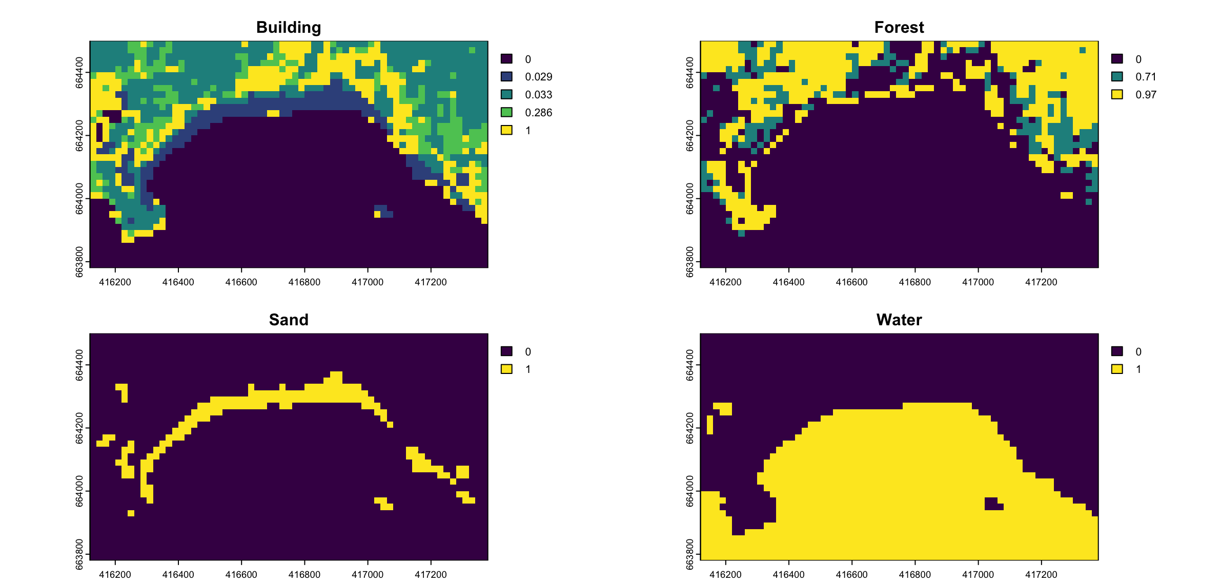
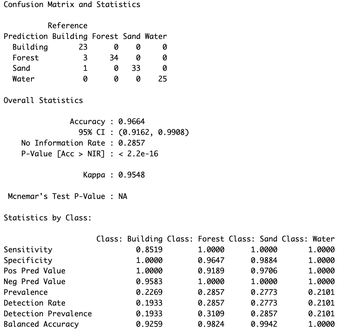
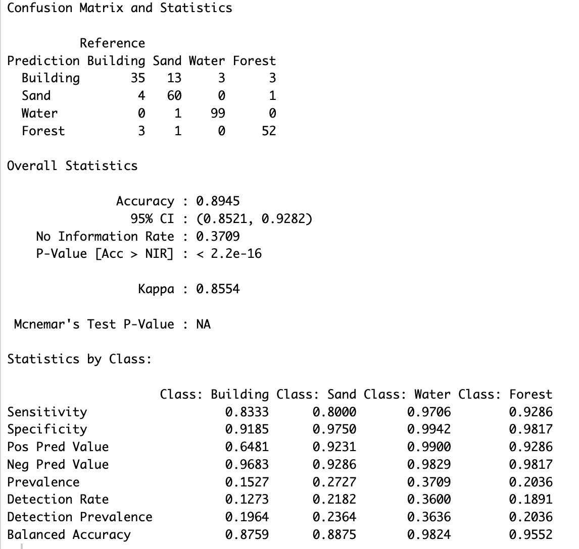
This demonstrates that the satellite data used in the project is capable of distinguishing between classes, even at a resolution of 20 meters. This confirms that the selected satellite data is suitable for further steps in the project. To quantify this, the confusion matrix generated from the CART model is analyzed, as illustrated in Figure 4.2. As anticipated, since the same image used for training was also used for evaluation, the accuracy is relatively high, with a value of 0.96%.
The CART model performs particularly well in predicting Sand, correctly classifying 33 points. The Building class was misclassifying 4 times. However, the model shows limitations in distinguishing between Building and Forest.
To understand why the CART model struggles to differentiate between Building and Forest, the decision tree was analyzed. It is also essential to identify which bands were utilized for the predictions to determine which ones provide the most valuable information. The CART model selected Bands 02, 05, 06, and 07 from the available set, indicating that these bands currently hold the most significant information for the given training dataset.
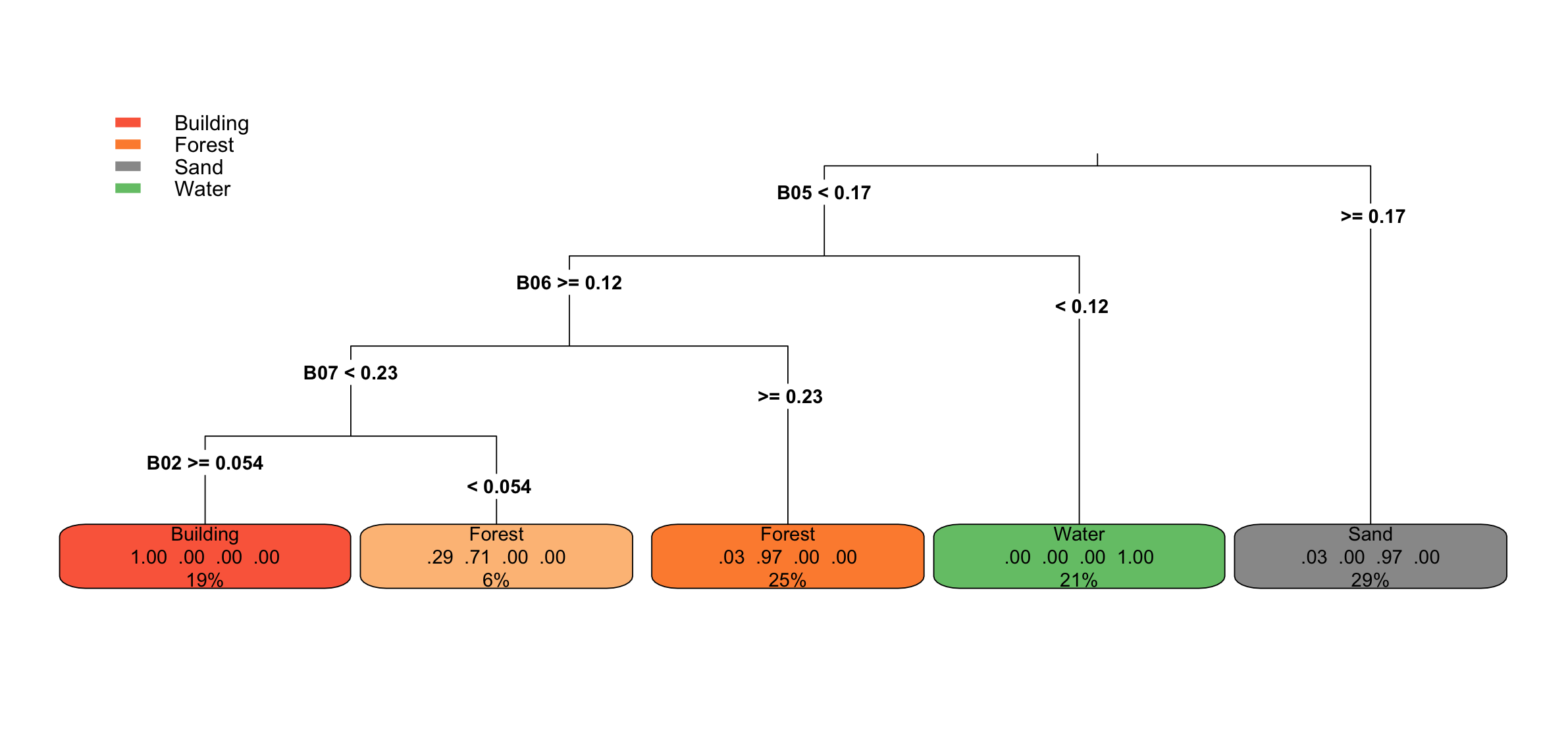
The Building class is predicted in the leftmost leaf node. In this node, the model predicts Building with 100% confidence (1.00 in the matrix). However, this node only accounts for 19% of the total data, suggesting that the Building class is not well-represented across the training dataset. This limited representation might contribute to the model’s difficulty in accurately distinguishing between Building and other classes, such as Forest.
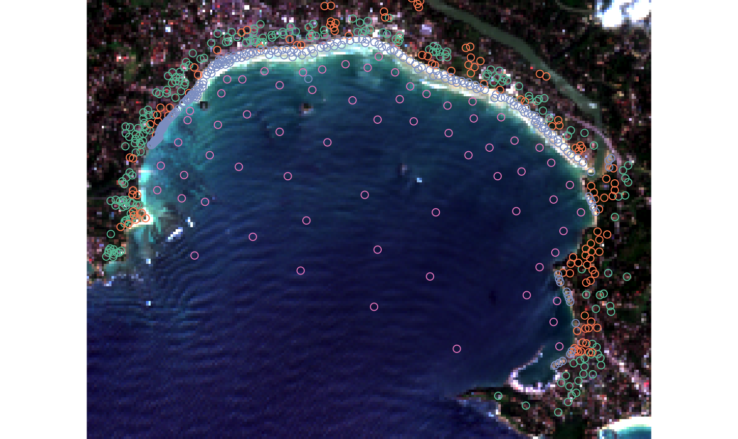
The performance of the trained CART model was evaluated on a different area within the same satellite image, separate from the region used for training. This visualization displays in Figure 4.4 the labeled data for Beach 1, showing the different classes overlaid on the RGB image. A substantial number of labels were created to evaluate the reliability and performance of the CART model.
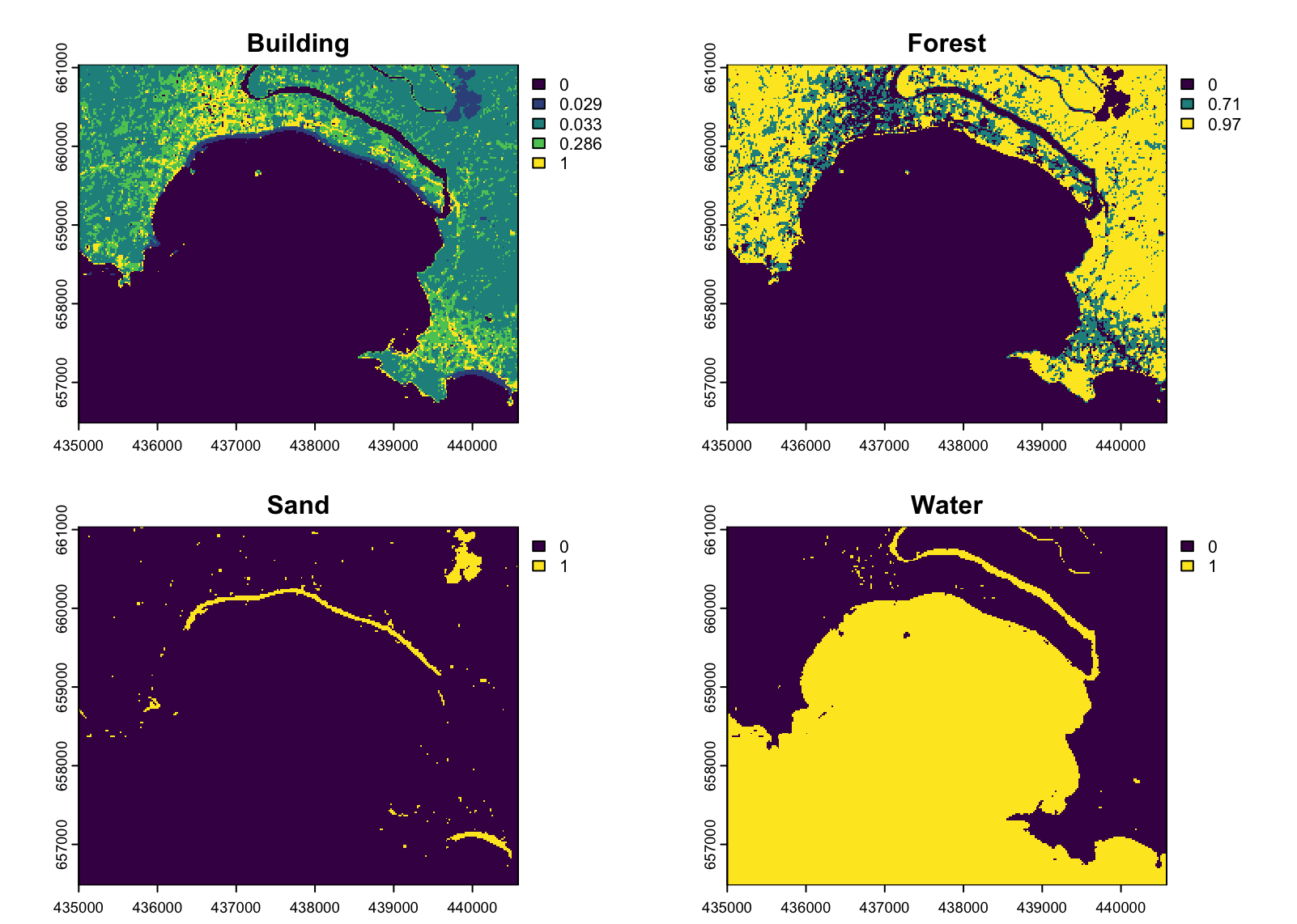
This visualization in Figure 4.5 presents the predictions for Beach 1 using the pre-trained model. In the upper section of the visualization, the Building and Forest classes are represented, while the lower section shows the classification results for Sand and Water. Sand and Water were reclassified for clarity, with Sand assigned a value of 1 and Water reclassified accordingly. The Sand class is generally well-predicted, with distinct regions along the coast accurately classified as Sand. These areas align with expected locations, showing high confidence in the model’s predictions. However, some regions where Sand was anticipated are not represented in the graph, indicating areas where the model’s performance could be improved. The Water class is also well-predicted, with clear and well-defined boundaries distinguishing water bodies from other land cover types. Most areas identified as Water were classified with high confidence, including the river visible in the image, which was delineated effectively.
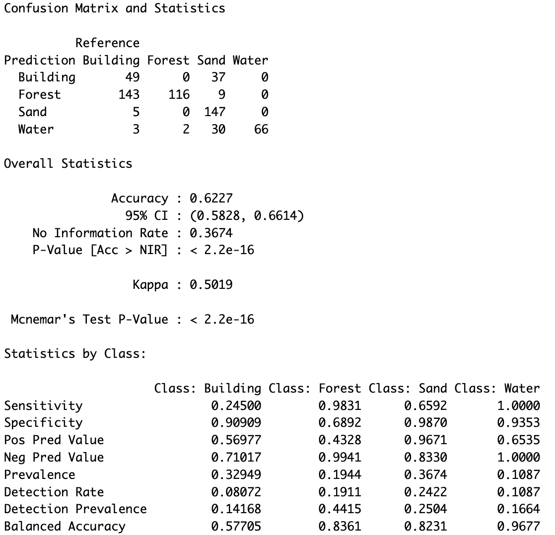
To evaluate the accuracy of the CART model on Beach Area 1, a confusion matrix was generated, illustrated in fig-Cart-Confusionmatrix-BEach-1. The overall performance of the model is limited, with an accuracy of 0.6227, indicating moderate classification capabilities.
The model struggles particularly with predicting the Sand class, which is the most critical class in this analysis. With a sensitivity of 0.6592, the model correctly classifies approximately 66% of the Sand pixels. This highlights the need for improvement in detecting Sand more effectively.
4.2 Evaluation Random Forest model
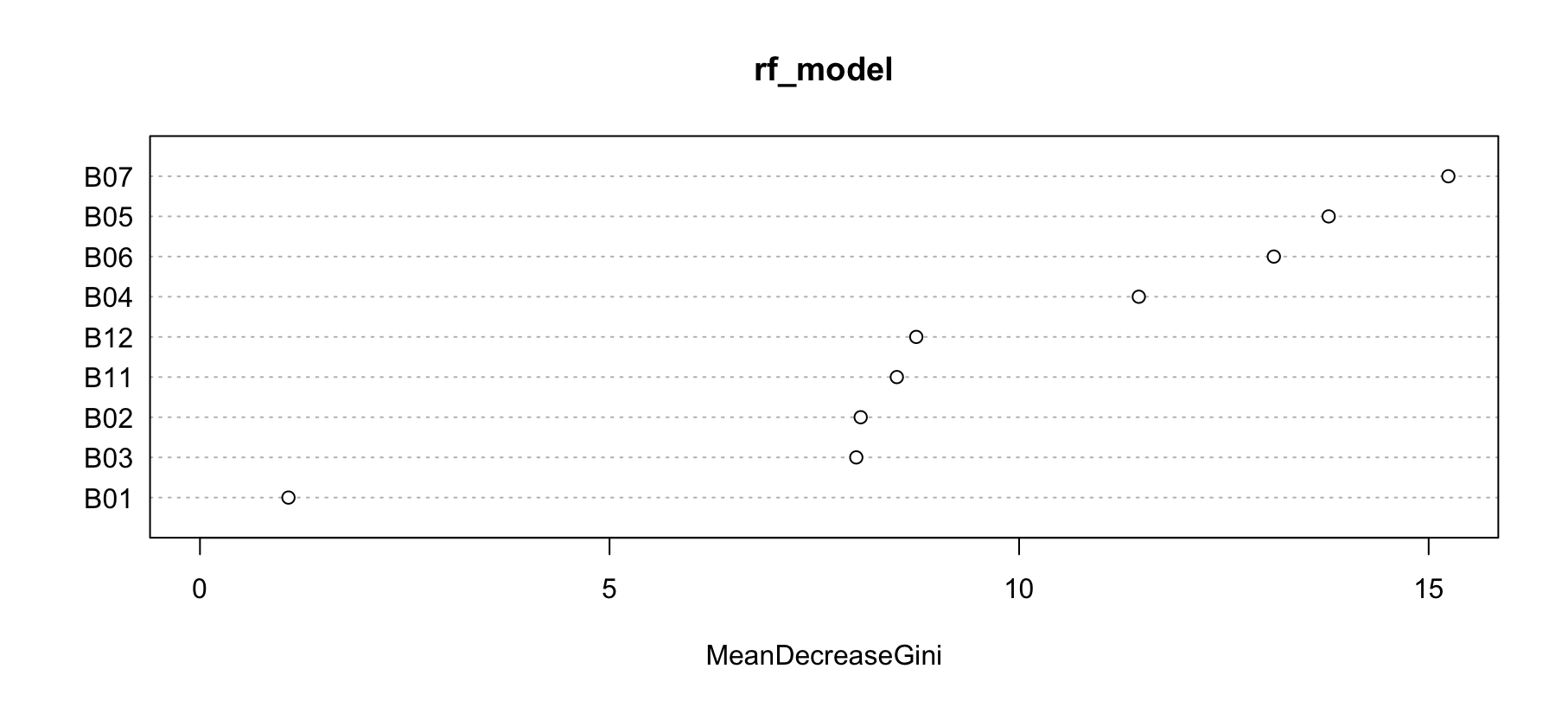
The Random Forest model, compared to the CART model, utilizes information from all available bands but prioritizes specific bands for classification, demonstrated in Figure 4.7. The feature importance analysis highlights which bands contribute the most to the model’s decision-making process. The Mean Decrease Gini metric is used to measure the importance of each band, indicating its role in reducing impurity in the decision trees.
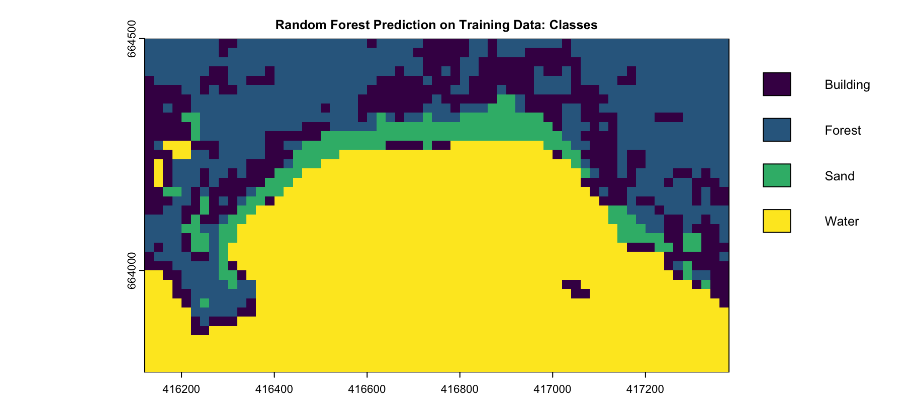
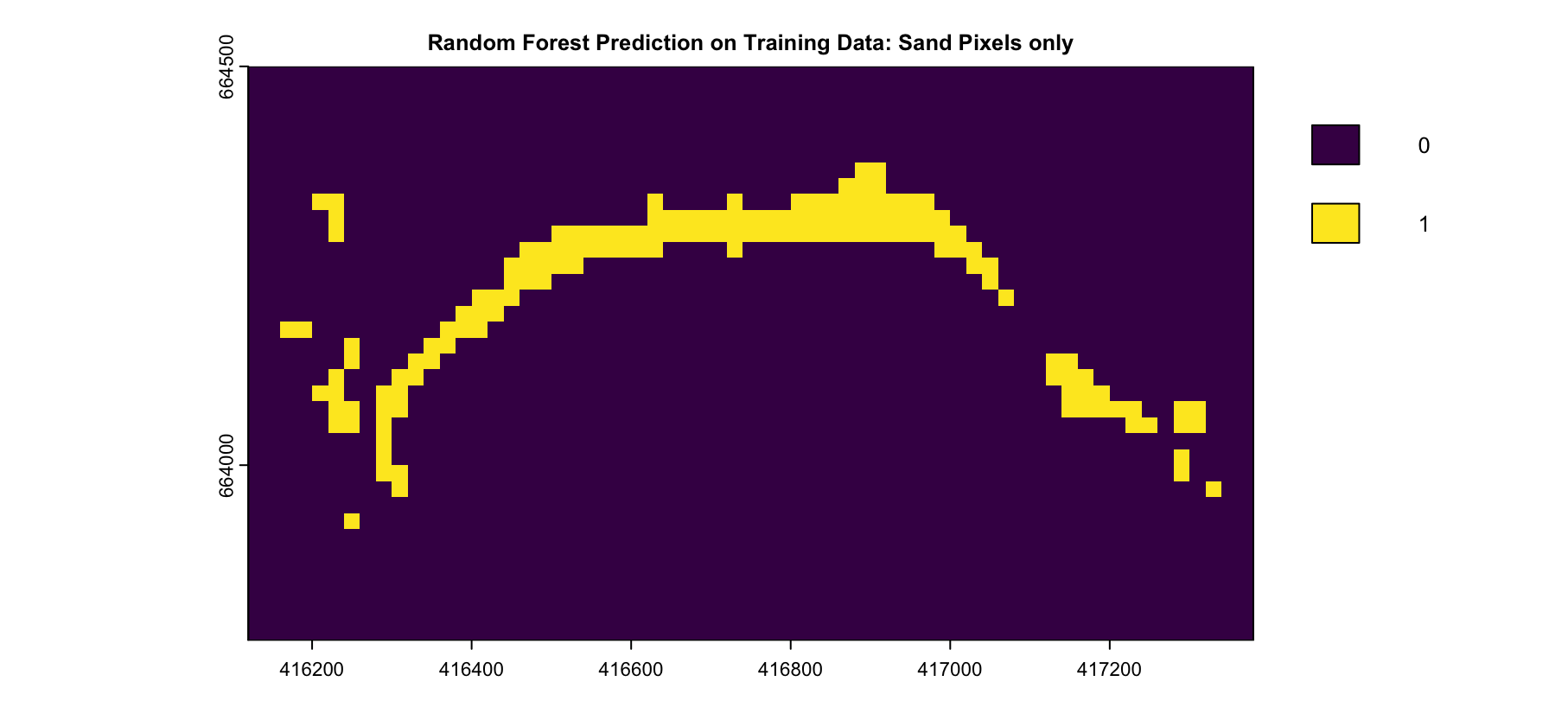
The Random Forest model was applied to the training dataset to classify land cover types, with a focus on the Sand class, in Figure 4.13 (a), shows the predicted classes, with Sand clearly distinguished along the coastal regions. However, some misclassifications between Buildings and Sand are visible, particularly in areas near the coastline. This is further illustrated in Figure 28, which isolates the Sand class, highlighting the areas identified as Sand by the model. These results demonstrate the model’s ability to classify Sand accurately within the training dataset while noting some limitations in distinguishing between Buildings and Sand.
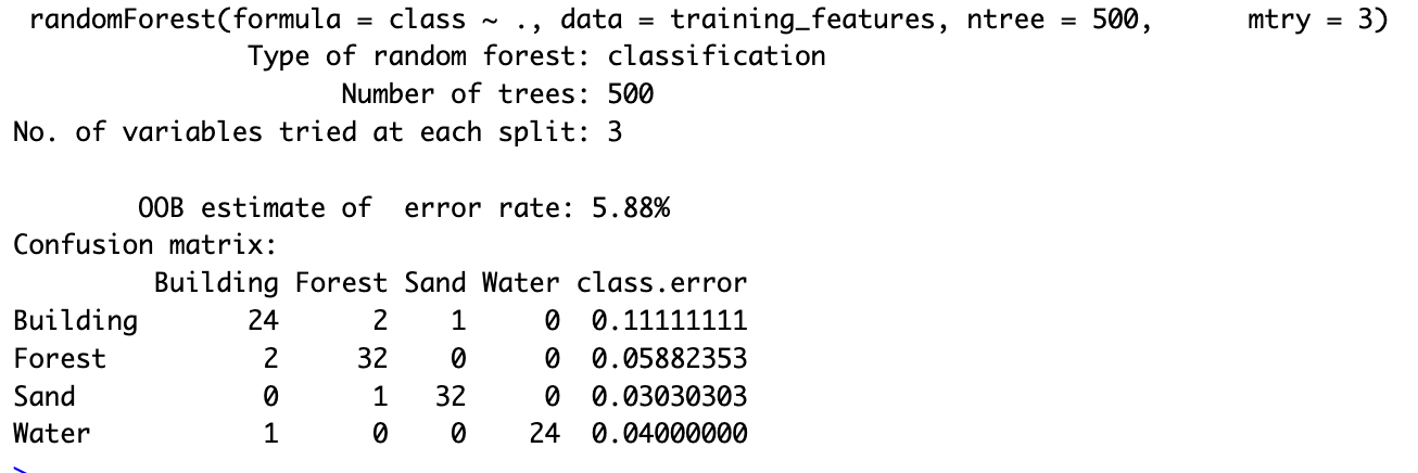
The confusion matrix highlights the performance of the Random Forest model trained and tested on the same labeled dataset. As expected, the model achieved a low out-of-bag (OOB) error rate of 5.88%, reflecting the consistency between the training data and predictions due to the reuse of the same image.
Focusing on the Sand class, which is the primary interest of this analysis, the model performed exceptionally well. It correctly classified 32 Sand pixels with only 1 misclassification, resulting in a class error rate of 3.03%. This demonstrates the model’s strong capability in identifying Sand as a distinct class, validating its suitability for this specific task.
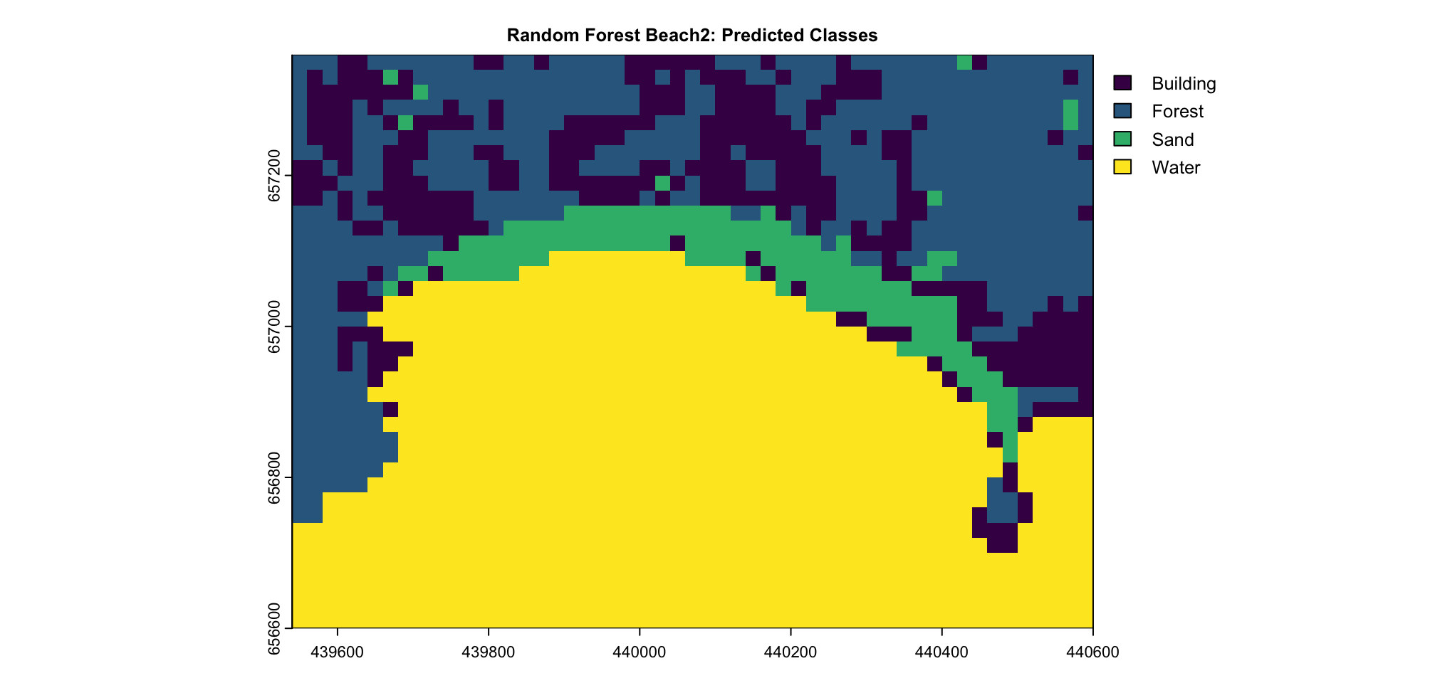
The Random Forest model, trained on labeled data, was applied to two distinct areas, Beach1 and Beach2, illustrated in Figure 4.10. These areas exhibit significantly different results in terms of classification accuracy and differentiation. Beach1 is compared to Beach2 a larger area.
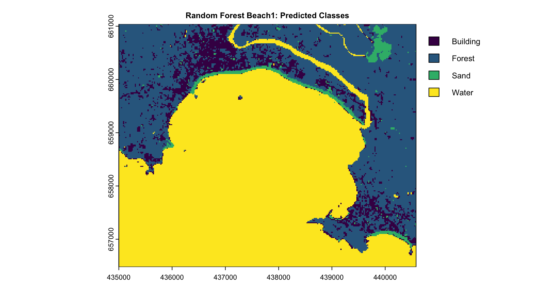
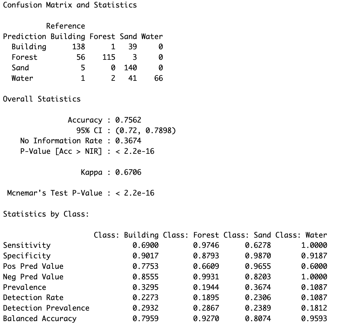
For Beach1, as shown in Figure 4.11 (a), the model achieved an overall accuracy of 75.62%, with a sensitivity of 62.78% for the Sand class. This means that approximately 63% of the actual Sand pixels were correctly identified, while 37.22% were misclassified. While the model demonstrates a moderate ability to detect Sand, there is clear room for improvement in sensitivity. On the other hand, the specificity for Sand is remarkably high at 98.70%, indicating that the model accurately classified 98.70% of No-Sand pixels as not Sand, effectively minimizing false positives. Additionally, the positive predictive value (PPV) for Sand is strong at 96.55%, meaning that when the model predicts Sand, it is correct 96.55% of the time. The balanced accuracy, which combines sensitivity and specificity, is 80.74%, reflecting an overall well-balanced performance for this class.
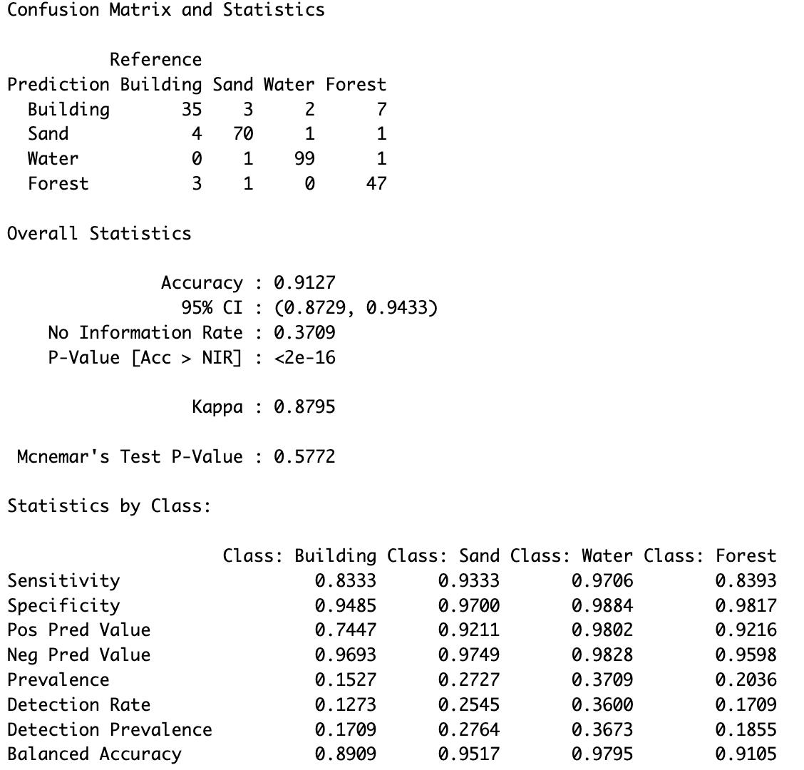
In contrast, Beach2, as shown in Figure 4.11 (b), which is smaller and less diverse than Beach1, yielded significantly better results, with an overall accuracy of 91.27%. The Sand class achieved an impressive sensitivity of 93.33%, successfully identifying the vast majority of Sand pixels. This high sensitivity, coupled with a specificity of 97.00% and a PPV of 92.11%, demonstrates the model’s robust performance in distinguishing Sand in this area. The improved results for Beach2 can likely be attributed to its clearer class boundaries and reduced landscape complexity, which make classification easier and more accurate.
It is also important to note the impact of dataset imbalance. The training data had fewer labeled points for the Building class compared to other classes, such as Sand and Water. This imbalance may have influenced the model’s ability to generalize effectively, particularly for Buildings, as seen in its lower sensitivity for this class.
In conclusion, the Random Forest model demonstrates strong performance in identifying Sand, with high specificity and PPV for both areas. However, the sensitivity for Sand in Beach1 highlights the need for further improvement to ensure more Sand pixels are correctly detected. Addressing dataset imbalances, especially for underrepresented classes like Buildings, could further enhance the model’s performance.
4.3 Evaluation Support Vector Machine
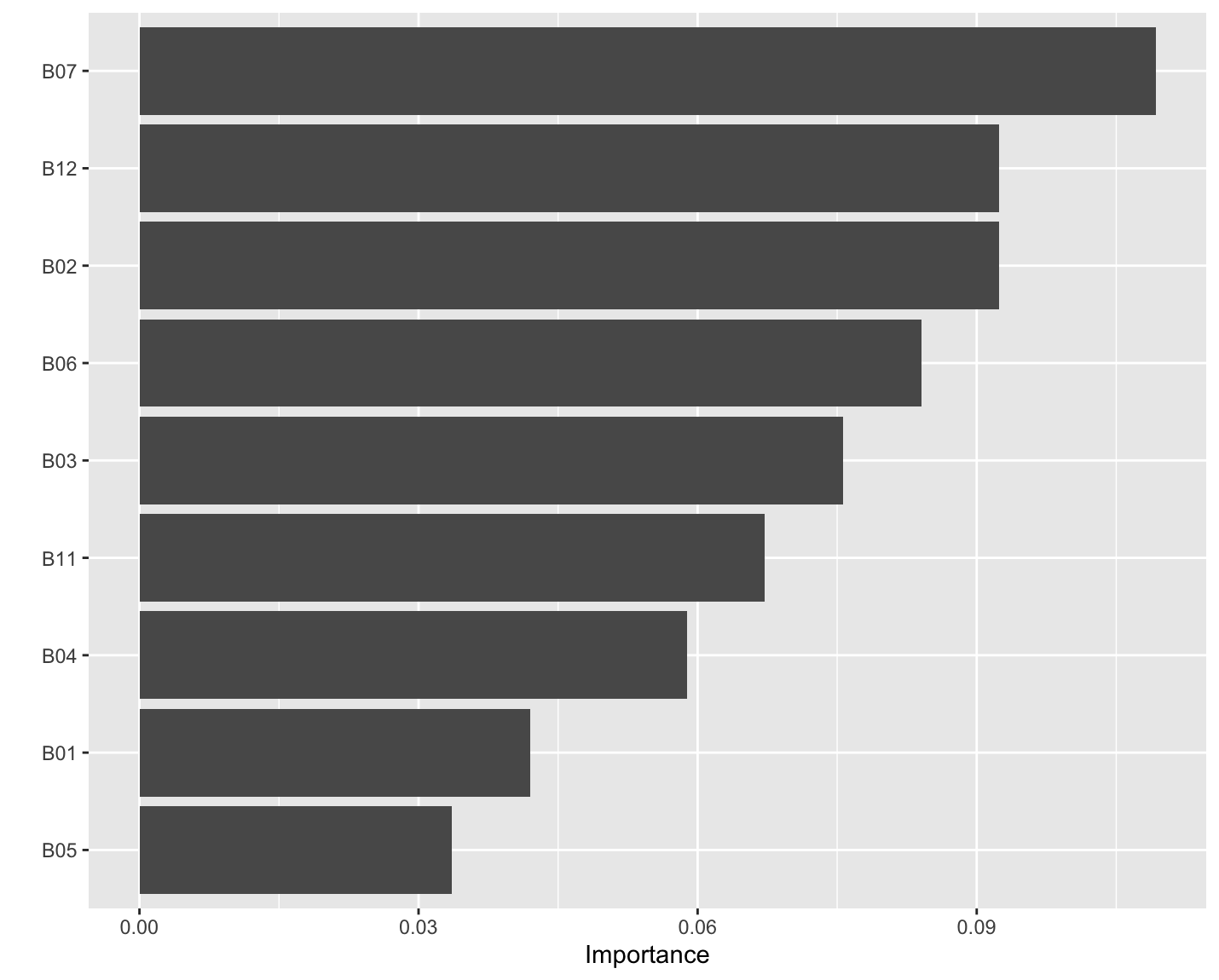
The SVM model utilized multiple spectral bands to classify Sand and other land cover types, as illustrated in Figure 4.12. An analysis of feature importance revealed that Bands B07, B12, and B02 played the most significant roles in the classification process. These bands contributed the highest to the model’s decision-making, suggesting that they contain the most relevant spectral information for distinguishing Sand from other classes. The importance of Bands B06 and B03 also indicates their complementary role in improving classification accuracy.
This result aligns with the expectation that near-infrared and shortwave infrared bands, such as B07 and B12, are particularly effective for detecting Sand and vegetation boundaries. However, the results also highlight the limitations of Sentinel-2 data, as these critical bands are only available at a 20 meter resolution, restricting the model’s potential for finer scale classifications.
The Support Vector Machine model was evaluated on Beach1 and Beach2 to analyze its performance, visualized in Figure 4.13. The results reveal considerable differences in the model’s performance between the two areas, which was also mentioned in the CART and Random Forest model.
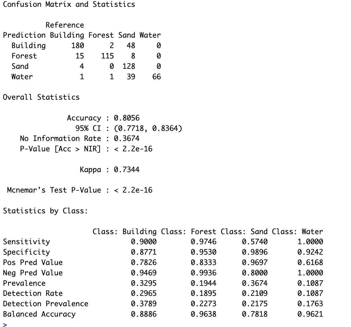
On Beach1, the model struggles with detecting Sand, achieving a sensitivity of 57.40%. This indicates that a significant portion of actual Sandpixels is misclassified into other categories. Despite this, the positive predictive value (PPV) for Sand is exceptionally high at 96.97%, meaning that when the model predicts Sand, it is accurate nearly all the time. The specificity for Sand is also high with 98.60%, showing that No-Sand pixels are rarely misclassified as Sand. However, the overall balanced accuracy for the Sand class is 78.18%, highlighting the need for improved detection in larger, more diverse areas like Beach1.
In contrast, Beach2 demonstrates significantly better results for the Sand class. The sensitivity improves to 80.00%, meaning the majority of Sand pixels are correctly identified. The PPV remains high at 92.31%, and the balanced accuracy rises to 88.75%. These results suggest that the SVM model performs better in the smaller, less complex area of Beach2, where class boundaries are more distinct and the landscape diversity is reduced.
Overall, the Support Vector Machine demonstrates strong performance in detecting Sand. However, there is room for improvement in distinguishing Sand more effectively from the Building and Water classes, which could potentially be achieved by incorporating more training data for these two classes.
4.4 Unawatuna Beach sand changes over time (2019–2023)
The evaluation of the Random Forest model reveals that it performs well on data that closely resembles the training dataset. This is evident in its ability to accurately predict Sand along the coastline, particularly in areas with features and shapes similar to those in the training data. This suggests that the model is reliable for analyzing timeline changes, as the consistent features of Unawatuna Beach over the years align well with the training data characteristics.
The sand area calculations were derived using Sentinel-2 data with a 20m resolution, where each pixel represents a 20m x 20m area. In the visualized results, shown in Figure 4.15, the model not only detects the sand coastline but also identifies sandy patches within urban and vegetative regions, which is a common feature in Sri Lankan coastal landscapes.
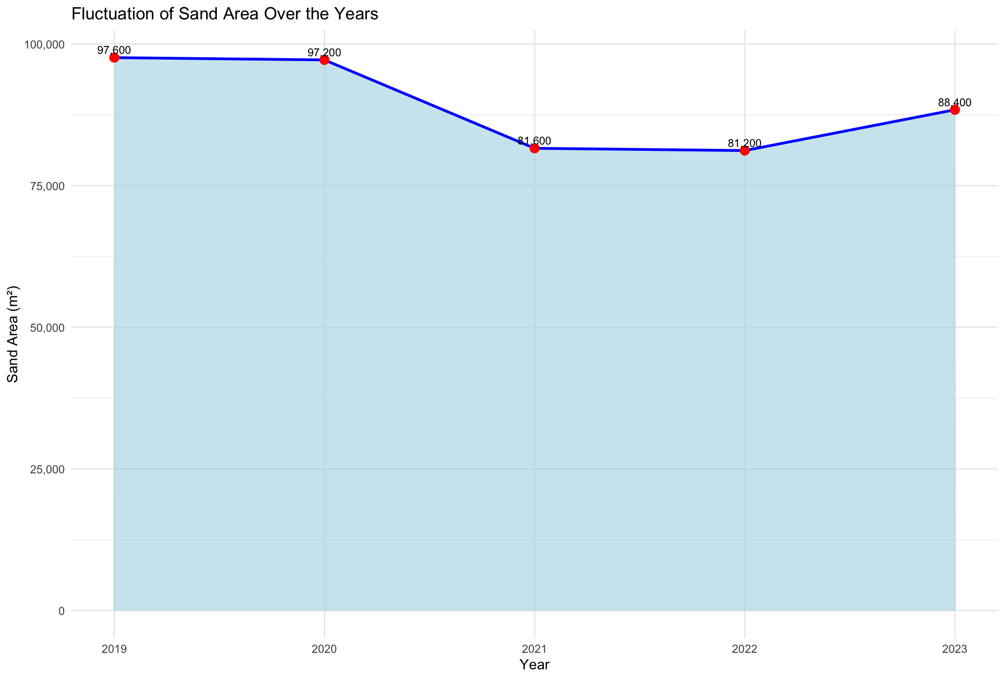
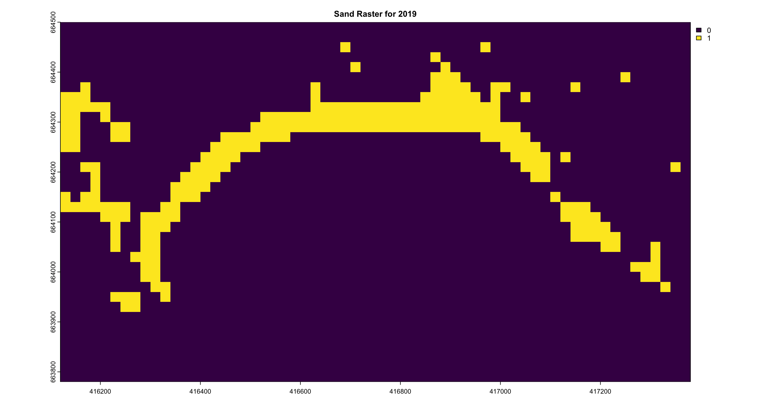
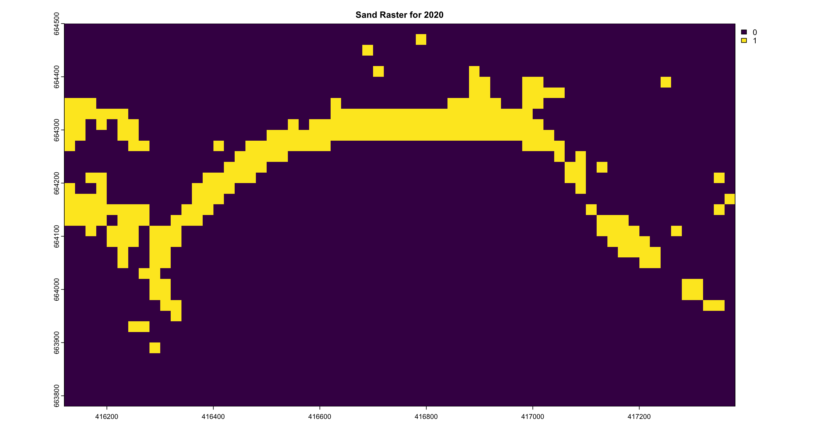
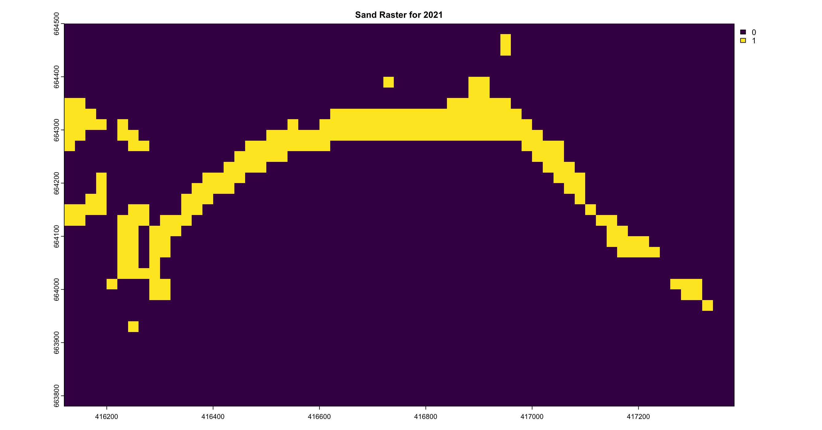
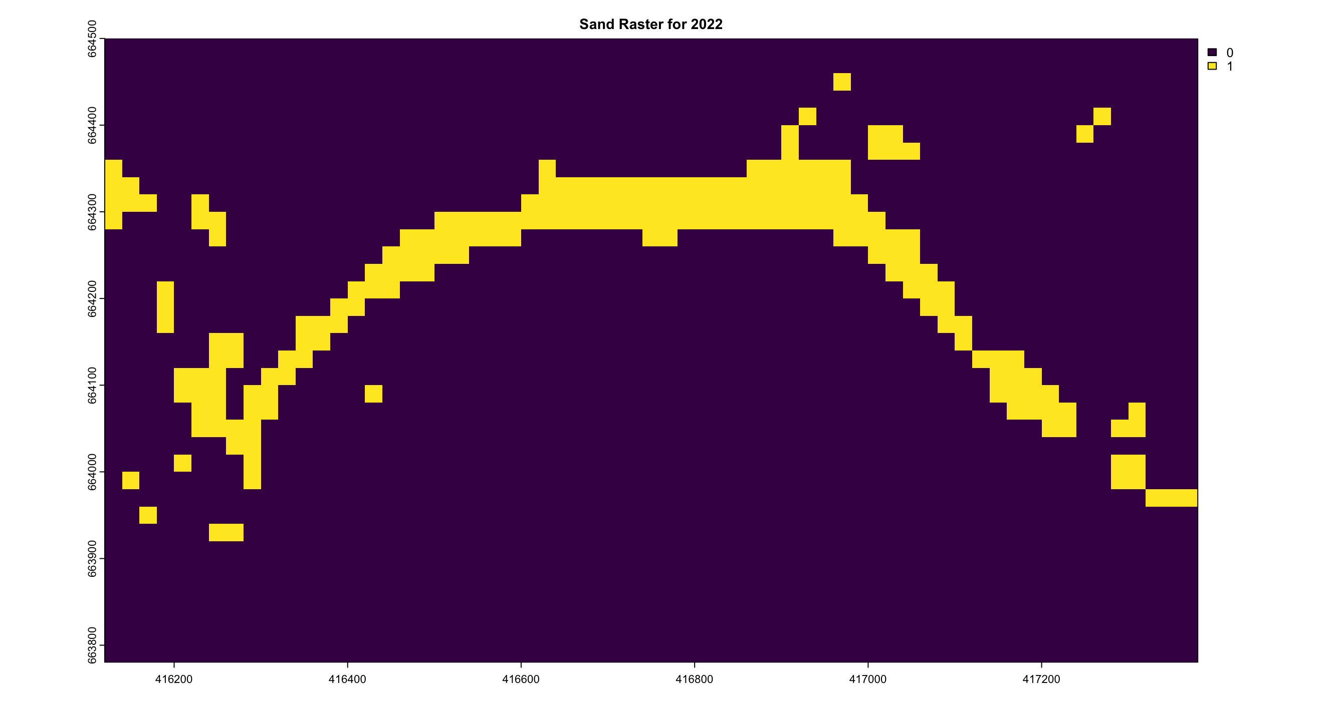
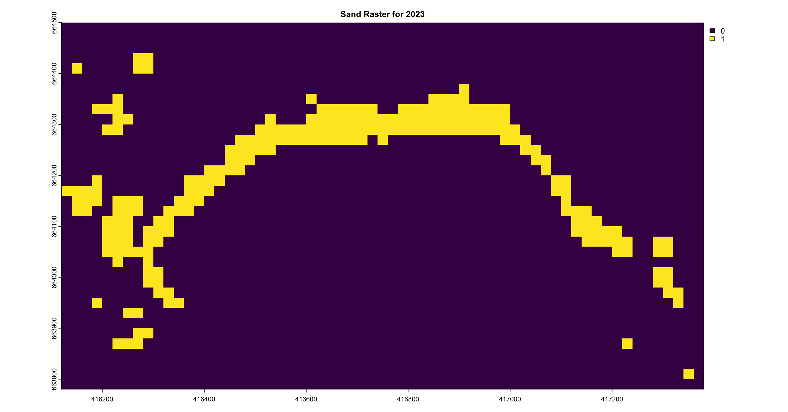
The analysis reveals a clear trend of decreasing sand levels between the years 2020 and 2021, as depicted in Figure 4.14, indicating a period of reduction in sand coverage along the shoreline. In contrast, the years 2022 and 2023 show a slight recovery, with an increase in sand levels compared to the preceding period. This fluctuation highlights the dynamic nature of sand distribution over time, with periods of both decline and recovery evident in the observed data. Table 4.1 shows the structed results of the pixel count.
| Year | Sand Area |
|---|---|
| 2019 | 97600 |
| 2020 | 97200 |
| 2021 | 81600 |
| 2022 | 81200 |
| 2023 | 88400 |